Kernel convolutions from scratch

Author

Jieming You

Published

October 10, 2022

Notebook for self-learning and playing with convolution matrices and applying them to raster inmages. All convolutions and matrices calculated and performed using base R.

library(jpeg)
set.seed(123)

Loading the image

Reading the image from a jpg file into a raster array. The image is loaded into an array of (500, 500, 3).

# Reading the sample image
img <- readJPEG("wall.jpg", native = FALSE)
dim(img)

[1] 500 500   3

Plotting the the raster image.

plotting function

plot_raster <- function(raster) {
  par(mfrow = c(1,1), mar = c(1,1,1,1))
  plot.new()
  as.raster(raster) |>
    rasterImage(xleft = 0, xright = 1, ytop = 0, ybottom = 1)
}

plot_raster(img)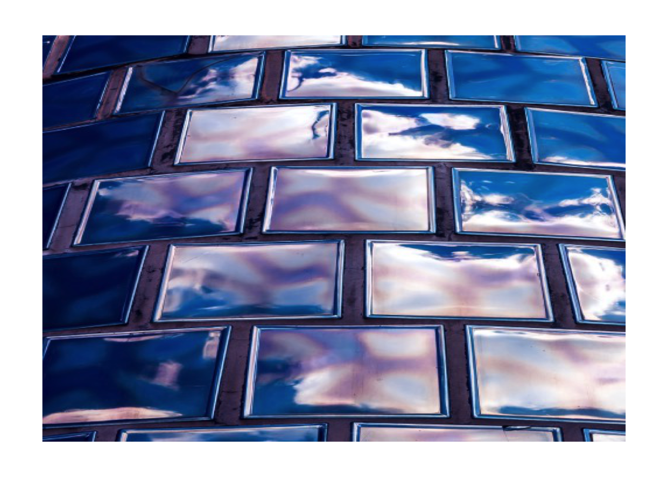

Convolving kernel

The convolution can be expressed as \[ g(x,y) = M \cdot f(x,y) = \sum_{dx=-a}^{a} \sum_{dy=-b}^{b} M(dx, dy) f(x-dx, y-dy) \]

That is, we calculate a new value for each pixel using the product of the convolution kernel and matrix of the same dimension from array f, in a rolling basis.

However, the edge pixels might cause problems when using a large kernel, as there are no adjacent pixels. This can be handled by edge padding.

Extended edge padding

In order to calculate convolutions also for the edge pixels, we can extend the edges by repeating edge values indefinitely.

Padding edge pixels by extension (Michael 2013).

The following function repeats the edge pixels of a given matrix for a specified mount of times.

edge_extension <- function(mat, pad) {
    n <- nrow(mat)
    m <- ncol(mat)

    top   <- c(rep(mat[1,1], pad), mat[1,], rep(mat[1,m], pad))
    bot   <- c(rep(mat[n,1], pad), mat[n,], rep(mat[n,m], pad))
    left  <- matrix(rep(mat[1:n, 1], pad), ncol=pad)
    right <- matrix(rep(mat[1:n, m], pad), ncol=pad)
    mid   <- cbind(left, mat[1:n,], right)

    new_mat <- rbind(
        matrix(rep(top, pad), nrow=pad, byrow=TRUE),
        mid,
        matrix(rep(bot, pad), nrow=pad, byrow=TRUE)
    )
    
    return(new_mat)
}

The function in action when given a following 3x3 matrix as input \[ \begin{bmatrix} 1 & 2 & 3 \\ 4 & 5 & 6 \\ 7 & 8 & 9 \end{bmatrix} \]

edge_extension(matrix(1:9, ncol=3, byrow=T), pad=2) |>
  write.table(row.names=F, col.names=F)

1 1 1 2 3 3 3
1 1 1 2 3 3 3
1 1 1 2 3 3 3
4 4 4 5 6 6 6
7 7 7 8 9 9 9
7 7 7 8 9 9 9
7 7 7 8 9 9 9

Applying the function

The following function calculates the rolling kernel using edge extension

rolling_kernel <- function(f, M) {
  
  x <- ncol(f)
  y <- nrow(f)
  m <- ncol(M)
  n <- nrow(M)
  g <- f # g(x,y)
  
  # Kernel dimensions exceed the source
  if (m > x ||  n  > y) {
    stop("Kernel length exceeds the source")
  }
  
  g_extended <- edge_extension(f, (m-1))
  
  for (i in 1:x) {
    for (j in 1:y) {
      f_kernel <- g_extended[i:(i+(m-1)), j:(j+(n-1))]
      g_kernel <- f_kernel * M
      g[i, j] <- sum(g_kernel)
    }
  }

  return(g)
}

A main wrapper function that convolves the given kernel for all three channels of an RGB-image. We have to also scale the values into [0,1] by computing \(\frac{\mathrm{rank}(A_{m \times n})}{m \cdot n}\).

rgb_kernel <- function(raster, kernel) {
  channels <- dim(raster)[3]
  output <- raster

  for (ch in 1:channels) {
    output[,,ch] <- rolling_kernel(raster[,,ch], kernel)
  }

  # Scaling
  output_reshape <- matrix(output, nrow = ncol(raster))
  output_scaled  <- rank(output_reshape) / length(output_reshape)
  dim(output_scaled) <- c(dim(raster))
  
  return(output_scaled)
}

Testing out common kernels

# Sharpen
img |>
  rgb_kernel(matrix(c(0,-1,0,-1,5,-1,0,-1,0), nrow=3)) |>
  plot_raster()

# Edge detection  
img |>
  rgb_kernel(matrix(c(-1,-1,-1,-1,8,-1,-1,-1,-1), nrow=3)) |>
  plot_raster()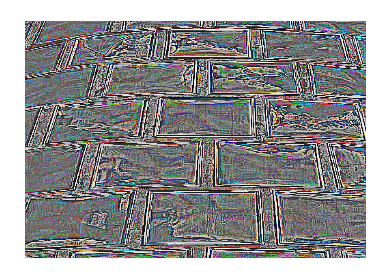

# Box blur
img |>
  rgb_kernel(matrix(rep(1, 81), nrow=9)) |>
  plot_raster()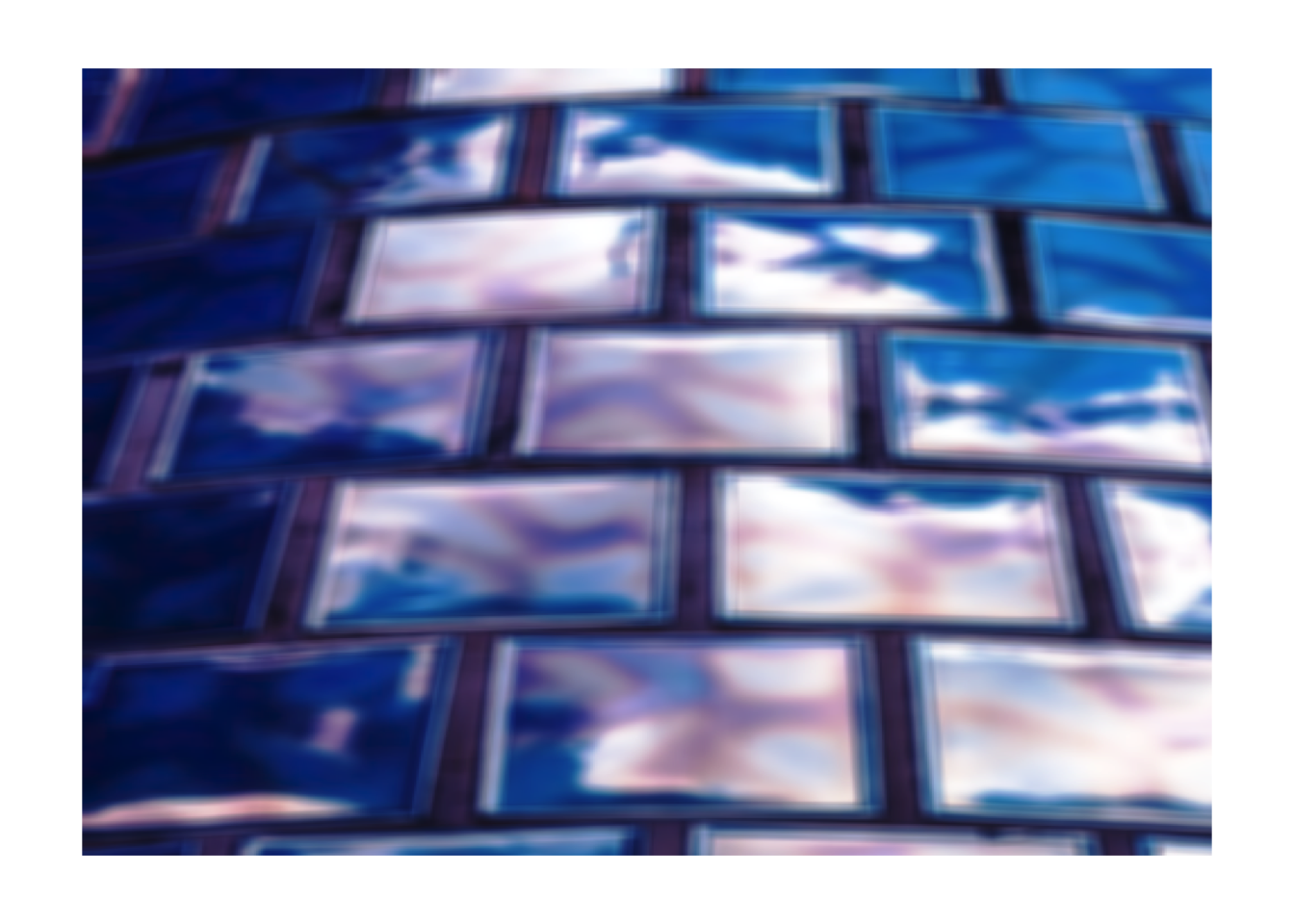

2-D Gaussian kernel

Gaussian blur can be applied by running a convolution using a Gaussian kernel. The two-dimensional Guaissian kernel is defined as \[ G(x,y) = \frac{1}{2 \pi \sigma ^2} e^{- \frac{x^2 + y^2}{2 \sigma ^2}} \]

Using the CDF of normal distribution, we can calculate the convolution matrix by

Generating a linspace \(u = \texttt{linspace}[\texttt{a}, \texttt{b}] \in \mathbb{R}^n\)
Using \(u\) to draw values from the Gaussian \(\texttt{CDF}\)
Calculating the convolution matrix \(M\) by taking the outer product \(M = uu^\top \in \mathbb{R}^{n \times n}\)

# Gaussian kernel function
gaussian_kernel <- function(width, sigma = 1) {
    if (width%%2 != 1) { stop("Even width parameter") }

    # Boundaries
    b  <- (width-1)/2
    a <- -b
    
    # Setting up the linspace
    ax <- seq(a, b, length = width)

    # Draw from gaussian CDF
    u <- dnorm(ax, sd = sigma)

    # Outer product uu^T and normalization
    M <- u %o% u
    M <- M / sum(M)

    return(M)
}

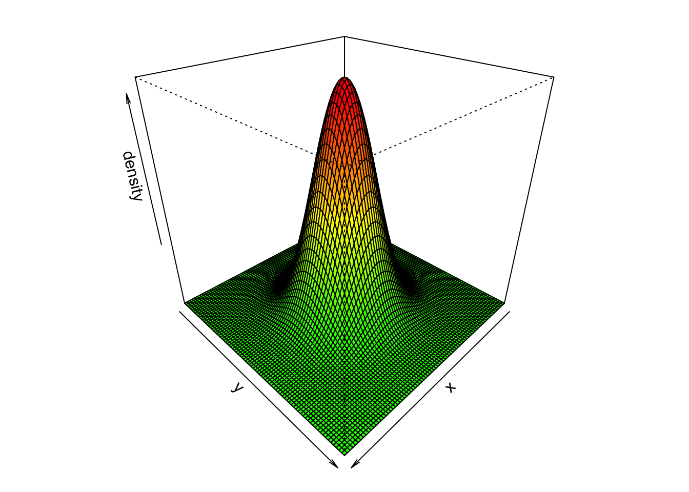
Plotting an example convolution matrix using width = 81 and sigma = 10.

Calculating color values for the plot

# Modified from: https://stackoverflow.com/a/39118422
z <- gaussian_kernel(width = 81, sigma = 10)
colors <- colorRampPalette(c("green", "yellow", "red"))(100)

z.facet.range <- ((z[-1, -1] +
                   z[-1, -ncol(z)] +
                   z[-nrow(z), -1] +
                   z[-nrow(z), -ncol(z)]) / 4) |>
                
                cut(100)

# Preparing the variables
M <- gaussian_kernel(width = 81, sigma = 10)
x <- y <- seq(-40, 40, length = 81)

# Plotting the 3D surface
par(mfrow = c(1,1), mar = c(1,1,1,1))
persp(x, y, M,
    theta = 135, phi = 30,
    zlab = "density",
    col = colors[z.facet.range]
)

3-D representation of the 2-D gaussian convolution

Gaussian blurring

Finally, convolving the gaussian kernel and applying a Gaussian Blurof radius: 40 and sd: 10.

# Gaussian blur
img |>
  rgb_kernel(gaussian_kernel(width = 81, sigma = 10)) |>
  plot_raster()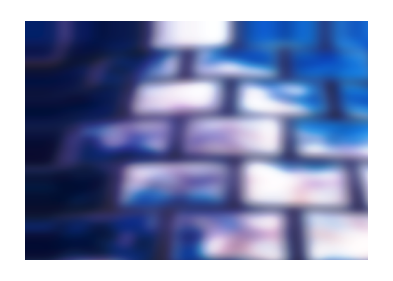

References

Michael, Plotke. 2013. Image Kernel Convolution, Extend Edge-Handling. Wikipedia. https://en.wikipedia.org/wiki/File:Extend_Edge-Handling.png.