import numpy as np
import pandas as pd
import matplotlib.pyplot as plt
import seaborn as sns

from itertools import groupby, combinations
from copy import deepcopy
from math import *
import random
import ast

from sklearn.model_selection import train_test_split
from sklearn.ensemble import RandomForestRegressor
from sklearn.metrics import mean_squared_error, r2_score

sns.set_theme(style="white")Assortment and Pricing Optimization using Random forest regressor
IE4214 Pricing Analytics and Revenue Management Group Project (modified)
Pricing
Machine Learning
This course project introduces a method for modeling product choice probability within a product assortment using Random Forest Regressor.
The IE4214 Revenue Management and Pricing Analytics course was taken in National Univesrity of Singapore, AY22/23.
The full final report can be read here: Link
Below is a slightly modified exceprt from the feature engineering chapter proposing a new way of creating features for assortment optimisation problems.
Introduction
This report analyzes a pricing and assortment optimization problem by solving several tasks. The problem consists of 5 different stock-keeping-units (SKUs): \([a,b,c,d,e,f]\). Each SKU has 5 different price levels: \([3000, 2700, 2400, 2100, 1800]\), meaning that there are 30 unique products in total.
A dataset assortment.txt is provided where each line in the dataset represents an assortment containing a set of the above-mentioned SKUs, with each SKU having one of the five price levels. In the dataset, the 30 products are assigned a number from 1 to 30 by ordering the products from SKU \(a\) to \(f\). Furthermore, within each SKU, the products are ordered from the highest to the lowest price level. For example, SKU \(b\) with the price 2700 will be represented as the number 7. In total, there are 2500 assortments.
| assortments.txt | |
|---|---|
| 0 | [0, 2] |
| 1 | [0, 22, 27] |
| 2 | [0, 7, 17, 22] |
| 3 | [0, 17, 7, 21, 14] |
| 4 | [0, 7, 2, 25, 30, 13] |
Another dataset probability.txt is provided which has an identical structure. However, this dataset represents the choice probability of a product in the assortment instead of the product itself. In order to solve the tasks related to this problem, these datasets must first be preprocessed, which is elaborated in the following section.
| probabilities.txt | |
|---|---|
| 0 | [0.617, 0.383] |
| 1 | [0.49, 0.386, 0.124] |
| 2 | [0.174, 0.448, 0.298, 0.08] |
| 3 | [0.134, 0.193, 0.365, 0.047, 0.261] |
| 4 | [0.095, 0.426, 0.023, 0.155, 0.003, 0.298] |
Data preparation
The provided data are first read from the text files.
assort_temp = []
prob_temp = []
with open("assortment.txt","r") as f, open("probability.txt","r") as g:
    for line1, line2 in zip(f, g):
        assort_temp.append(ast.literal_eval(line1))
        prob_temp.append(ast.literal_eval(line2))
As the original dataset contains duplicate rows, they are removed before any further data processing. Moreover, as the customer choice model appears to be determinisitic, the duplicates will not provide additional information about the customers’ choice logic.
# Removes duplicates
def remove_duplicates(lst):
    seen = []
    for i in lst:
        if i not in seen:
            seen.append(i)
    return seen
assort = remove_duplicates(assort_temp)
prob = remove_duplicates(prob_temp)Our aim is to create a model that predicts the choice probability of a product given the other products in the assortment.
Instead of predicting the choice distribution of the whole assortment, it would be easier to predict the choice probability of a single product, given the other available products in the assortment.
For example, instead of coming up with a choice probability distribution for the assortment \([0, 5, 9]\), one might ask what is the probability of customer choosing product 5, given that the other options are not buying anything (0) and product 9.
The next subsections will cover the feature engineering and construction of the features and labels.
Labels
The choice probabilities provided in the probabilities.txt file are \(n\)-dimensional arrays with \(n\) discrete choice options. In order to simplify our model and reduce the amount of model training required, we reduced the dimension of the label space by splitting each array (choice probability distribution) into \(n\) distinct labels, each consisting of a single probability. This way, instead of predicting an array of probabilities, we are only predicting the choice probability of a single product.
\[ \begin{aligned} \text{original array} & & \text{labels} \\ \left[\textcolor{red}{0.4}, \textcolor{OliveGreen}{0.1}, \textcolor{blue}{0.5}\right] & \longrightarrow & [\textcolor{red}{0.4}] \\ && [\textcolor{OliveGreen}{0.1}] \\ &&[\textcolor{blue}{0.5}] \end{aligned} \]
Features
Each assortment array is also split into \(n\) feature vectors as follows; for each product in an assortment:
- Set the product as the first feature \(x_1\)
\[ \begin{aligned} \text{original array} & & \text{feature vectors} \\ \left[\textcolor{red}{0}, \textcolor{OliveGreen}{5}, \textcolor{blue}{9}\right] & \longrightarrow & [\textcolor{red}{0} \\ && [\textcolor{OliveGreen}{5}\\ && [\textcolor{blue}{9} \end{aligned} \]
- Encode the information of the other products in the assortment using multi-hot-encoding, also known as multi-label-binarizing
Because each assortment has varying amounts of products, the multi-hot-encoding is used to standardize the length of the feature vectors.
As there is an outside option and thirty (30) different products, the multi-label-binarizer has a shape of (1,31). For example, an assortment \([0,5,9]\) can be represented as
\[ \begin{aligned} \text{Assortment} \quad & [\textcolor{red}{0}, \textcolor{OliveGreen}{5}, \textcolor{blue}{9}]\\ \text{Multi-hot} \quad & [\textcolor{red}{1},0,0,0,0,\textcolor{OliveGreen}{1},0,0,0,\textcolor{blue}{1},0,0,0,0,0,0,0,0,0,0,0,0,0,0,0,0,0,0,0,0,0] \end{aligned} \]
Hence, the final feature vectors are
\[ \begin{aligned} \text{original array} && && \text{feature vectors}\\ [\textcolor{red}{0}, \textcolor{OliveGreen}{5}, \textcolor{blue}{9}] && \longrightarrow && [\textcolor{red}{0},~ (0, 0, 0, 0, 0, \textcolor{OliveGreen}{1}, 0, 0, 0, \textcolor{blue}{1}, 0, ..., 0)]\\ &&&& [\textcolor{OliveGreen}{5}, ~(\textcolor{red}{1}, 0, 0, 0, 0, 0, 0, 0, 0, \textcolor{blue}{1}, 0, ..., 0)]\\ &&&& [\textcolor{blue}{9}, ~(\textcolor{red}{1}, 0, 0, 0, 0, \textcolor{OliveGreen}{1}, 0, 0, 0, 0, 0, ..., 0)] \end{aligned} \]
After performing the transformations, we have a total of 8617 data points. The data points are finally split into separate training and testing sets. For the initial training, we will use the conventional 80-20 split and shuffle the datapoints to reduce the risk of overfitting.
TEST_SIZE = 0.2    # Size of test set
SHUFFLE = True     # Shuffle the datapoints
RANDOM_STATE = 42  # For reproducibility
Setting up the data
Functions used for the data transformation can be found at Appendix A.
Transforming the data and splitting it into training and testing set
# Splitting
X_train_raw, X_test_raw, y_train_raw, y_test_raw = train_test_split(
    assort, prob, test_size=TEST_SIZE, shuffle=SHUFFLE,
    random_state=RANDOM_STATE
)
# Constructing the features and lables
X_train, y_train = transform_data(X_train_raw, y_train_raw)
X_test, y_test = transform_data(X_test_raw, y_test_raw)Model
We have chosen to use the Random Forest Regressor from Scikit-learn to predict the numerical choice probabilities. A random forest is a set (ensemble) of different decision trees. Each of these decision trees is obtained by fitting a perturbed copy of the original dataset (Jung, 2022). Each decision tree then gives a prediction of the target variable and the final prediction is the average of all the predictions. The random forest regressor has been superior to, for example, a single decision tree or gradient tree boosting, because it handles outliers, missing values and overfitting better due to the averaging.
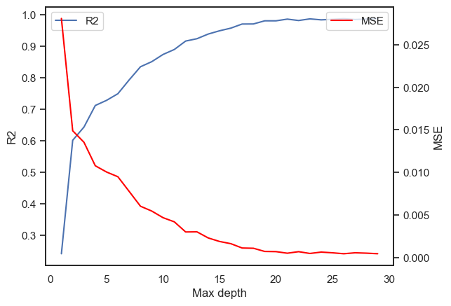
The main parameter in our model is the max depth parameter, which specifies the maximum depth of each decision tree from root node to leaf node. A deep node makes the model more complex and thus more prone to overfitting. In our case, we determined the optimal max depth by plotting it against \(R^2\) and MSE values (See Figure 1). We can see that the \(R^2\) and MSE values are converging when max depth is greater than 20. Thus, our model uses a max depth of 20.
We train the models using our training set and predict the choice probabilities using the test set.
# Initiating the model and model using training set
reg = RandomForestRegressor(max_depth = 20, random_state=RANDOM_STATE)
reg = reg.fit(X_train, y_train)
To make calculating the prediction easier, we created a wrapper function for prediction choice probabilitites given a product assortment and a choice model (in our case, the Random Forest Regressor).
def predict(assortment: list[int], model=reg) -> list[float]:
    X = transformX(assortment).tolist()
    y_pred = model.predict(X)
    y_pred_normalized = y_pred / sum(y_pred)
    return y_pred_normalized
Model evaluation
The model’s predictive performance is assessed by calculating the mean-squared-error (MSE) of the predictions.
# 1) Calculating the choice probabilities for the testing set
y_preds = [ predict(assortment) for assortment in X_test_raw]

# 2) Calculating the mean MSE
MSE_test = assortment_mse(y_preds, y_test_raw)
print(f"The average MSE for an assortment is {np.mean(MSE_test) :.2f} %pp")
print(f"The median MSE for an assortment is {np.median(MSE_test) :.2f} %pp")
The average MSE for an assortment is 1.46 %pp
The median MSE for an assortment is 0.51 %pp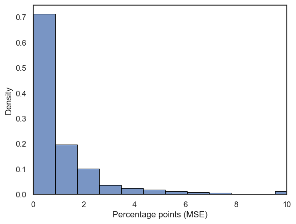
The model performs well when tested on the testing set. The average MSE of the prediction for an assortment is under two percentage points. Furthermore, the median MSE is under one percentage point which indicates excellent prediction accuracy.
As seen from Figure 2, the long tail of the histogram is the cause of the average MSE being significantly worse than the median MSE.
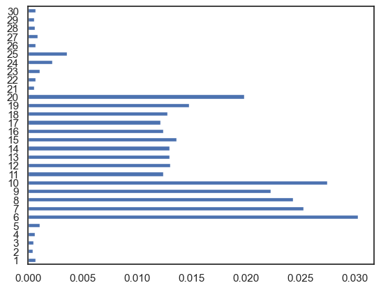
In addition to the MSE, we can evaluate the popularity of the products by calculating the feature importance for the multi-hot encoded array. If a feature is important, its value has a significant effect on the prediction. In other words, the products with the highest corresponding importance are the most sought after as their presence in the assortment have a signicant impact on the choice probability of the other product.
The feature importance of the produts are shown in Figure 3. Based on the observations, the products \(a\), \(e\), and \(f\) are less popular, whereas the products \(b\), \(c\), and \(d\) are more popular.
feat_imp = pd.Series(reg.feature_importances_[2:])
feat_imp.set_axis(range(1,31), inplace=True)
feat_imp.plot(kind='barh')
plt.show()